
Example n° 5: Optimizing and serving UAV data
In the previous example we have seen how useful it can be to compress an RGB formatted TIFF image and to embed compressed overviews in it.
When dealing with UAV (Unmanned Aerial Vehicles, commonly known as drone) aerial images it could be very useful to use tiles. Tiling allows large raster datasets to be broken-up into manageable pieces and are fundamental in defining and implementing an higher level raster I/O interface.
In this example we will use the original dataset of the chiangMai_ortho_optimized public raster layer which is currently available on the Thai CHIANG MAI Urban Flooding GeoNode platform (see the GeoNode documentation to read more about that).
This dataset contains an orthorectified image stored as RGBa GeoTiff with 4 bands, three bands for the RGB and one for transparency (the alpha channel).
Note
On a Windows machine you can set-up a shell with all GDAL Utilities, running directly the file OSGeo4W.bat under the %TRAINING_ROOT% folder.
Calling the gdalinfo command to see detailed information:
gdalinfo chiangMai_ortho.tif
It will produce the following results:
Driver: GTiff/GeoTIFF
Files: chiangMai_ortho.tif
Size is 63203, 66211
Coordinate System is:
PROJCS["WGS 84 / UTM zone 47N",
    GEOGCS["WGS 84",
        DATUM["WGS_1984",
            SPHEROID["WGS 84",6378137,298.257223563,
                AUTHORITY["EPSG","7030"]],
            AUTHORITY["EPSG","6326"]],
        PRIMEM["Greenwich",0,
            AUTHORITY["EPSG","8901"]],
        UNIT["degree",0.0174532925199433,
            AUTHORITY["EPSG","9122"]],
        AUTHORITY["EPSG","4326"]],
    PROJECTION["Transverse_Mercator"],
    PARAMETER["latitude_of_origin",0],
    PARAMETER["central_meridian",99],
    PARAMETER["scale_factor",0.9996],
    PARAMETER["false_easting",500000],
    PARAMETER["false_northing",0],
    UNIT["metre",1,
        AUTHORITY["EPSG","9001"]],
    AXIS["Easting",EAST],
    AXIS["Northing",NORTH],
    AUTHORITY["EPSG","32647"]]
Origin = (487068.774750000040513,2057413.889810000080615)
Pixel Size = (0.028850000000000,-0.028850000000000)
Metadata:
  AREA_OR_POINT=Area
  TIFFTAG_SOFTWARE=pix4dmapper
Image Structure Metadata:
  COMPRESSION=LZW
  INTERLEAVE=PIXEL
Corner Coordinates:
Upper Left  (  487068.775, 2057413.890) ( 98d52'38.72"E, 18d36'27.34"N)
Lower Left  (  487068.775, 2055503.702) ( 98d52'38.77"E, 18d35'25.19"N)
Upper Right (  488892.181, 2057413.890) ( 98d53'40.94"E, 18d36'27.38"N)
Lower Right (  488892.181, 2055503.702) ( 98d53'40.98"E, 18d35'25.22"N)
Center      (  487980.478, 2056458.796) ( 98d53' 9.85"E, 18d35'56.28"N)
Band 1 Block=63203x1 Type=Byte, ColorInterp=Red
  NoData Value=-10000
  Mask Flags: PER_DATASET ALPHA
Band 2 Block=63203x1 Type=Byte, ColorInterp=Green
  NoData Value=-10000
  Mask Flags: PER_DATASET ALPHA
Band 3 Block=63203x1 Type=Byte, ColorInterp=Blue
  NoData Value=-10000
  Mask Flags: PER_DATASET ALPHA
Band 4 Block=63203x1 Type=Byte, ColorInterp=Alpha
  NoData Value=-10000
As you can see, this GeoTiff has not been tiled. For accessing subsets though, tiling can make a difference. With tiling, data are stored and compressed in blocks (tiled) rather than line by line (stripped).
In the command output above it is visible that each band has blocks with the same width of the image (63203) and a unit length. The grids in the picture below show an image with equally sized tiles (left) and the same number of strips (right). To read data from the red subset, the intersected area will have to be decompressed.
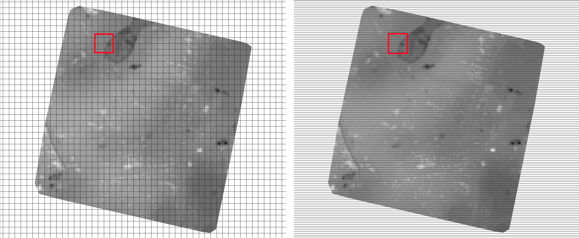
In the tiled image we will have to decompress only 16 tiles, whereas in the stripped image on the right we’ll have to decompress many more strips.
Drone images data usually have a stripped structure so, in most cases, they need to be optimized to increase performances. Let’s take a look at the gdal_translate command used to optimize our GeoTiff:
gdal_translate -co TILED=YES -co COMPRESS=JPEG -co PHOTOMETRIC=YCBCR
               --config GDAL_TIFF_INTERNAL_MASK YES -b 1 -b 2 -b 3 -mask 4
               chiangMai_ortho.tif
               chiangMai_ortho_optimized.tif
The parameters are:
TILED=YES: forces the creation of a tiled output GeoTiff with default parameters (BLOCKXSIZE=256 and BLOCKYSIZE=256 creation options)COMPRESS=JPEG: activates the JPEG compression with the default parameters (RGB photometric interpretation and a quality of 75%)PHOTOMETRIC=YCBCR: switches the photometric interpretation to the yCbCr color space, which allows a significant further reduction in output size with minimal changes on the imagesGDAL_TIFF_INTERNAL_MASK YES: creates an internal transparency mask that contains 1 sample of 1-bit data (1-bit internal mask band are deflate compressed); when reading the mask back, to make conversion between mask band and alpha band easier, its bands are exposed to the user as being promoted to full 8 bits (i.e. the value for unmasked pixels is 255) unless the GDAL_TIFF_INTERNAL_MASK_TO_8BIT configuration option is set to NO (this does not affect the way the mask band is written, it is always 1-bit)-b 1 -b 2 -b 3: writes three bands on the output files based on the set of input bands (bands can be also reordered)-mask 4: creates an output mask band from the fourth input band (bands are numbered from 1)
Once the process ended, call the gdalinfo command on the resulting tif file:
gdalinfo chiangMai_ortho_optimized.tif
The following should be the results:
Driver: GTiff/GeoTIFF
Files: chiangMai_ortho_optimized.tif
Size is 63203, 66211
Coordinate System is:
PROJCS["WGS 84 / UTM zone 47N",
    GEOGCS["WGS 84",
        DATUM["WGS_1984",
            SPHEROID["WGS 84",6378137,298.257223563,
                AUTHORITY["EPSG","7030"]],
            AUTHORITY["EPSG","6326"]],
        PRIMEM["Greenwich",0,
            AUTHORITY["EPSG","8901"]],
        UNIT["degree",0.0174532925199433,
            AUTHORITY["EPSG","9122"]],
        AUTHORITY["EPSG","4326"]],
    PROJECTION["Transverse_Mercator"],
    PARAMETER["latitude_of_origin",0],
    PARAMETER["central_meridian",99],
    PARAMETER["scale_factor",0.9996],
    PARAMETER["false_easting",500000],
    PARAMETER["false_northing",0],
    UNIT["metre",1,
        AUTHORITY["EPSG","9001"]],
    AXIS["Easting",EAST],
    AXIS["Northing",NORTH],
    AUTHORITY["EPSG","32647"]]
Origin = (487068.774750000040513,2057413.889810000080615)
Pixel Size = (0.028850000000000,-0.028850000000000)
Metadata:
  AREA_OR_POINT=Area
  TIFFTAG_SOFTWARE=pix4dmapper
Image Structure Metadata:
  COMPRESSION=YCbCr JPEG
  INTERLEAVE=PIXEL
  SOURCE_COLOR_SPACE=YCbCr
Corner Coordinates:
Upper Left  (  487068.775, 2057413.890) ( 98d52'38.72"E, 18d36'27.34"N)
Lower Left  (  487068.775, 2055503.702) ( 98d52'38.77"E, 18d35'25.19"N)
Upper Right (  488892.181, 2057413.890) ( 98d53'40.94"E, 18d36'27.38"N)
Lower Right (  488892.181, 2055503.702) ( 98d53'40.98"E, 18d35'25.22"N)
Center      (  487980.478, 2056458.796) ( 98d53' 9.85"E, 18d35'56.28"N)
Band 1 Block=256x256 Type=Byte, ColorInterp=Red
  NoData Value=-10000
  Mask Flags: PER_DATASET
Band 2 Block=256x256 Type=Byte, ColorInterp=Green
  NoData Value=-10000
  Mask Flags: PER_DATASET
Band 3 Block=256x256 Type=Byte, ColorInterp=Blue
  NoData Value=-10000
  Mask Flags: PER_DATASET
Our GeoTiff is now tiled with 256x256 tiles, has 3 bands and a 1-bit mask for nodata.
We can also add internal overviews to the file using the gdaladdo command:
gdaladdo -r average chiangMai_ortho_optimized.tif 2 4 8 16 32 64 128 256 512
gdal_translate command), so the parameters to be specified are:-r average: computes the average of all non-NODATA contributing pixels2 4 8 16 32 64 128 256 512: the list of integral overview levels to build (from gdal version 2.3 levels are no longer required to build overviews)
Calling the gdalinfo command again:
gdalinfo chiangMai_ortho_optimized.tif
It results in:
Driver: GTiff/GeoTIFF
Files: chiangMai_ortho_optimized.tif
Size is 63203, 66211
Coordinate System is:
PROJCS["WGS 84 / UTM zone 47N",
    GEOGCS["WGS 84",
        DATUM["WGS_1984",
            SPHEROID["WGS 84",6378137,298.257223563,
                AUTHORITY["EPSG","7030"]],
            AUTHORITY["EPSG","6326"]],
        PRIMEM["Greenwich",0,
            AUTHORITY["EPSG","8901"]],
        UNIT["degree",0.0174532925199433,
            AUTHORITY["EPSG","9122"]],
        AUTHORITY["EPSG","4326"]],
    PROJECTION["Transverse_Mercator"],
    PARAMETER["latitude_of_origin",0],
    PARAMETER["central_meridian",99],
    PARAMETER["scale_factor",0.9996],
    PARAMETER["false_easting",500000],
    PARAMETER["false_northing",0],
    UNIT["metre",1,
        AUTHORITY["EPSG","9001"]],
    AXIS["Easting",EAST],
    AXIS["Northing",NORTH],
    AUTHORITY["EPSG","32647"]]
Origin = (487068.774750000040513,2057413.889810000080615)
Pixel Size = (0.028850000000000,-0.028850000000000)
Metadata:
  AREA_OR_POINT=Area
  TIFFTAG_SOFTWARE=pix4dmapper
Image Structure Metadata:
  COMPRESSION=YCbCr JPEG
  INTERLEAVE=PIXEL
  SOURCE_COLOR_SPACE=YCbCr
Corner Coordinates:
Upper Left  (  487068.775, 2057413.890) ( 98d52'38.72"E, 18d36'27.34"N)
Lower Left  (  487068.775, 2055503.702) ( 98d52'38.77"E, 18d35'25.19"N)
Upper Right (  488892.181, 2057413.890) ( 98d53'40.94"E, 18d36'27.38"N)
Lower Right (  488892.181, 2055503.702) ( 98d53'40.98"E, 18d35'25.22"N)
Center      (  487980.478, 2056458.796) ( 98d53' 9.85"E, 18d35'56.28"N)
Band 1 Block=256x256 Type=Byte, ColorInterp=Red
  NoData Value=-10000
  Overviews: 31602x33106, 15801x16553, 7901x8277, 3951x4139, 1976x2070, 988x1035, 494x518, 247x259, 124x130
  Mask Flags: PER_DATASET
  Overviews of mask band: 31602x33106, 15801x16553, 7901x8277, 3951x4139, 1976x2070, 988x1035, 494x518, 247x259, 124x130
Band 2 Block=256x256 Type=Byte, ColorInterp=Green
  NoData Value=-10000
  Overviews: 31602x33106, 15801x16553, 7901x8277, 3951x4139, 1976x2070, 988x1035, 494x518, 247x259, 124x130
  Mask Flags: PER_DATASET
  Overviews of mask band: 31602x3Results in:3106, 15801x16553, 7901x8277, 3951x4139, 1976x2070, 988x1035, 494x518, 247x259, 124x130
Band 3 Block=256x256 Type=Byte, ColorInterp=Blue
  NoData Value=-10000
  Overviews: 31602x33106, 15801x16553, 7901x8277, 3951x4139, 1976x2070, 988x1035, 494x518, 247x259, 124x130
  Mask Flags: PER_DATASET
  Overviews of mask band: 31602x33106, 15801x16553, 7901x8277, 3951x4139, 1976x2070, 988x1035, 494x518, 247x259, 124x130
Notice that the transparency masks of internal overviews have been applied (their compression does not show up in the file metadata).
UAVs usually provide also two other types of data: DTM (Digital Terrain Model) and DSM (Digital Surface Model).
Those data require different processes to be optimized.
Let’s look at some examples to better understand how to use gdal to accomplish that task.
From the CHIANG MAI Urban Flooding GeoNode platform it is currently available the chiangMai_dtm_optimized layer, let’s download its original dataset.
This dataset should contain the DTM file chiangMai_dtm.tif.
Calling the gdalinfo command on it:
gdalinfo chiangMai_dtm.tif
The following information will be displayed:
Driver: GTiff/GeoTIFF
Files: chiangMai_dtm.tif
Size is 12638, 13240
Coordinate System is:
PROJCS["WGS 84 / UTM zone 47N",
    GEOGCS["WGS 84",
        DATUM["WGS_1984",
            SPHEROID["WGS 84",6378137,298.257223563,
                AUTHORITY["EPSG","7030"]],
            AUTHORITY["EPSG","6326"]],
        PRIMEM["Greenwich",0,
            AUTHORITY["EPSG","8901"]],
        UNIT["degree",0.0174532925199433,
            AUTHORITY["EPSG","9122"]],
        AUTHORITY["EPSG","4326"]],
    PROJECTION["Transverse_Mercator"],
    PARAMETER["latitude_of_origin",0],
    PARAMETER["central_meridian",99],
    PARAMETER["scale_factor",0.9996],
    PARAMETER["false_easting",500000],
    PARAMETER["false_northing",0],
    UNIT["metre",1,
        AUTHORITY["EPSG","9001"]],
    AXIS["Easting",EAST],
    AXIS["Northing",NORTH],
    AUTHORITY["EPSG","32647"]]
Origin = (487068.774750000040513,2057413.889810000080615)
Pixel Size = (0.144270000000000,-0.144270000000000)
Metadata:
  AREA_OR_POINT=Area
  TIFFTAG_SOFTWARE=pix4dmapper
Image Structure Metadata:
  COMPRESSION=LZW
  INTERLEAVE=BAND
Corner Coordinates:
Upper Left  (  487068.775, 2057413.890) ( 98d52'38.72"E, 18d36'27.34"N)
Lower Left  (  487068.775, 2055503.755) ( 98d52'38.77"E, 18d35'25.19"N)
Upper Right (  488892.059, 2057413.890) ( 98d53'40.94"E, 18d36'27.37"N)
Lower Right (  488892.059, 2055503.755) ( 98d53'40.98"E, 18d35'25.22"N)
Center      (  487980.417, 2056458.822) ( 98d53' 9.85"E, 18d35'56.28"N)
Band 1 Block=12638x1 Type=Float32, ColorInterp=Gray
  NoData Value=-10000
Reading this image could be very slow because it has not been tiled yet. So, as discussed above, its data need to be stored and compressed in tiles to increase performances.
The following gdal_translate command should be appropriate for that purpose:
gdal_translate -co TILED=YES -co COMPRESS=DEFLATE chiangMai_dtm.tif chiangMai_dtm_optimized.tif
When the data to compress consists of imagery (es. aerial photographs, true-color satellite images, or colored maps) you can use lossy algorithms such as JPEG.
We are now compressing data where the precision is important, the band data type is Float32 and elevation values should not be altered, so a lossy algorithm such as JPEG is not suitable.
JPEG should generally only be used with Byte data (8 bit per channel) so we have choosen the lossless DEFLATE compression through the COMPRESS=DEFLATE creation option.
Calling the gdalinfo command again:
gdalinfo chiangMai_dtm_optimized.tif
We can observe the following results:
Driver: GTiff/GeoTIFF
Files: chiangMai_dtm_optimized.tif
Size is 12638, 13240
Coordinate System is:
PROJCS["WGS 84 / UTM zone 47N",
    GEOGCS["WGS 84",
        DATUM["WGS_1984",
            SPHEROID["WGS 84",6378137,298.257223563,
                AUTHORITY["EPSG","7030"]],
            AUTHORITY["EPSG","6326"]],
        PRIMEM["Greenwich",0,
            AUTHORITY["EPSG","8901"]],
        UNIT["degree",0.0174532925199433,
            AUTHORITY["EPSG","9122"]],
        AUTHORITY["EPSG","4326"]],
    PROJECTION["Transverse_Mercator"],
    PARAMETER["latitude_of_origin",0],
    PARAMETER["central_meridian",99],
    PARAMETER["scale_factor",0.9996],
    PARAMETER["false_easting",500000],
    PARAMETER["false_northing",0],
    UNIT["metre",1,
        AUTHORITY["EPSG","9001"]],
    AXIS["Easting",EAST],
    AXIS["Northing",NORTH],
    AUTHORITY["EPSG","32647"]]
Origin = (487068.774750000040513,2057413.889810000080615)
Pixel Size = (0.144270000000000,-0.144270000000000)
Metadata:
  AREA_OR_POINT=Area
  TIFFTAG_SOFTWARE=pix4dmapper
Image Structure Metadata:
  COMPRESSION=DEFLATE
  INTERLEAVE=BAND
Corner Coordinates:
Upper Left  (  487068.775, 2057413.890) ( 98d52'38.72"E, 18d36'27.34"N)
Lower Left  (  487068.775, 2055503.755) ( 98d52'38.77"E, 18d35'25.19"N)
Upper Right (  488892.059, 2057413.890) ( 98d53'40.94"E, 18d36'27.37"N)
Lower Right (  488892.059, 2055503.755) ( 98d53'40.98"E, 18d35'25.22"N)
Center      (  487980.417, 2056458.822) ( 98d53' 9.85"E, 18d35'56.28"N)
Band 1 Block=256x256 Type=Float32, ColorInterp=Gray
  NoData Value=-10000
We need also to create overviews through the gdaladdo command:
gdaladdo -r nearest chiangMai_dtm_optimized.tif 2 4 8 16 32 64
Unlike the previous example, overviews will be created with the nearest resampling algorithm.
That is due to the nature of the data we are representing: we should not consider the average between two elevation values but simply the closer one, it is more reliable regarding the conservation of the original data.
Calling the gdalinfo command again:
gdalinfo chiangMai_dtm_optimized.tif
We can see the following information:
Driver: GTiff/GeoTIFF
Files: chiangMai_dtm_optimized.tif
Size is 12638, 13240
Coordinate System is:
PROJCS["WGS 84 / UTM zone 47N",
    GEOGCS["WGS 84",
        DATUM["WGS_1984",
            SPHEROID["WGS 84",6378137,298.257223563,
                AUTHORITY["EPSG","7030"]],
            AUTHORITY["EPSG","6326"]],
        PRIMEM["Greenwich",0,
            AUTHORITY["EPSG","8901"]],
        UNIT["degree",0.0174532925199433,
            AUTHORITY["EPSG","9122"]],
        AUTHORITY["EPSG","4326"]],
    PROJECTION["Transverse_Mercator"],
    PARAMETER["latitude_of_origin",0],
    PARAMETER["central_meridian",99],
    PARAMETER["scale_factor",0.9996],
    PARAMETER["false_easting",500000],
    PARAMETER["false_northing",0],
    UNIT["metre",1,
        AUTHORITY["EPSG","9001"]],
    AXIS["Easting",EAST],
    AXIS["Northing",NORTH],
    AUTHORITY["EPSG","32647"]]
Origin = (487068.774750000040513,2057413.889810000080615)
Pixel Size = (0.144270000000000,-0.144270000000000)
Metadata:
  AREA_OR_POINT=Area
  TIFFTAG_SOFTWARE=pix4dmapper
Image Structure Metadata:
  COMPRESSION=DEFLATE
  INTERLEAVE=BAND
Corner Coordinates:
Upper Left  (  487068.775, 2057413.890) ( 98d52'38.72"E, 18d36'27.34"N)
Lower Left  (  487068.775, 2055503.755) ( 98d52'38.77"E, 18d35'25.19"N)
Upper Right (  488892.059, 2057413.890) ( 98d53'40.94"E, 18d36'27.37"N)
Lower Right (  488892.059, 2055503.755) ( 98d53'40.98"E, 18d35'25.22"N)
Center      (  487980.417, 2056458.822) ( 98d53' 9.85"E, 18d35'56.28"N)
Band 1 Block=256x256 Type=Float32, ColorInterp=Gray
  NoData Value=-10000
  Overviews: 6319x6620, 3160x3310, 1580x1655, 790x828, 395x414, 198x207
Overviews have been created.
By default, they inherit the same compression type of the original dataset (there is no evidence of it in the gdalinfo output).
The CHIANG MAI Urban Flooding GeoNode platform makes also available the chiangMai_dsm_optimized layer’s original dataset for downloading.
This should contain the DSM file chiangMai_dsm.tif.
DTM is simply an elevation surface representing the bare earth referenced to a common vertical datum, a DSM is very similar to it but it captures the natural and built features on the Earth’s surface.
They both represent the same data type so those two datasets can be treated in the same way.Checking the file current configuration with gdalinfo:
gdalinfo chiangMai_dsm.tif
The following information should be displayed:
Driver: GTiff/GeoTIFF
Files: chiangMai_dsm.tif
Size is 63203, 66211
Coordinate System is:
PROJCS["WGS 84 / UTM zone 47N",
    GEOGCS["WGS 84",
        DATUM["WGS_1984",
            SPHEROID["WGS 84",6378137,298.257223563,
                AUTHORITY["EPSG","7030"]],
            AUTHORITY["EPSG","6326"]],
        PRIMEM["Greenwich",0,
            AUTHORITY["EPSG","8901"]],
        UNIT["degree",0.0174532925199433,
            AUTHORITY["EPSG","9122"]],
        AUTHORITY["EPSG","4326"]],
    PROJECTION["Transverse_Mercator"],
    PARAMETER["latitude_of_origin",0],
    PARAMETER["central_meridian",99],
    PARAMETER["scale_factor",0.9996],
    PARAMETER["false_easting",500000],
    PARAMETER["false_northing",0],
    UNIT["metre",1,
        AUTHORITY["EPSG","9001"]],
    AXIS["Easting",EAST],
    AXIS["Northing",NORTH],
    AUTHORITY["EPSG","32647"]]
Origin = (487068.774750000040513,2057413.889810000080615)
Pixel Size = (0.028850000000000,-0.028850000000000)
Metadata:
  AREA_OR_POINT=Area
  TIFFTAG_SOFTWARE=pix4dmapper
Image Structure Metadata:
  COMPRESSION=LZW
  INTERLEAVE=BAND
Corner Coordinates:
Upper Left  (  487068.775, 2057413.890) ( 98d52'38.72"E, 18d36'27.34"N)
Lower Left  (  487068.775, 2055503.702) ( 98d52'38.77"E, 18d35'25.19"N)
Upper Right (  488892.181, 2057413.890) ( 98d53'40.94"E, 18d36'27.38"N)
Lower Right (  488892.181, 2055503.702) ( 98d53'40.98"E, 18d35'25.22"N)
Center      (  487980.478, 2056458.796) ( 98d53' 9.85"E, 18d35'56.28"N)
Band 1 Block=63203x1 Type=Float32, ColorInterp=Gray
  NoData Value=-10000
Calling gdal_translate to apply tiling and compression:
gdal_translate -co TILED=YES -co COMPRESS=DEFLATE -co BIGTIFF=YES chiangMai_dsm.tif chiangMai_dsm_optimized.tif
Note
We used the BIGTIFF=YES creation option because the file is larger than 4 GB. Alternatively, the BIGTIFF=IF_NEEDED will only create a BigTIFF if it is clearly needed. The BIGTIFF=IF_SAFER will create BigTIFF if the resulting file might exceed 4GB.
Calling gdalinfo again:
gdalinfo chiangMai_dsm_optimized.tif
Results:
Driver: GTiff/GeoTIFF
Files: chiangMai_dsm_optimized.tif
Size is 63203, 66211
Coordinate System is:
PROJCS["WGS 84 / UTM zone 47N",
    GEOGCS["WGS 84",
        DATUM["WGS_1984",
            SPHEROID["WGS 84",6378137,298.257223563,
                AUTHORITY["EPSG","7030"]],
            AUTHORITY["EPSG","6326"]],
        PRIMEM["Greenwich",0,
            AUTHORITY["EPSG","8901"]],
        UNIT["degree",0.0174532925199433,
            AUTHORITY["EPSG","9122"]],
        AUTHORITY["EPSG","4326"]],
    PROJECTION["Transverse_Mercator"],
    PARAMETER["latitude_of_origin",0],
    PARAMETER["central_meridian",99],
    PARAMETER["scale_factor",0.9996],
    PARAMETER["false_easting",500000],
    PARAMETER["false_northing",0],
    UNIT["metre",1,
        AUTHORITY["EPSG","9001"]],
    AXIS["Easting",EAST],
    AXIS["Northing",NORTH],
    AUTHORITY["EPSG","32647"]]
Origin = (487068.774750000040513,2057413.889810000080615)
Pixel Size = (0.028850000000000,-0.028850000000000)
Metadata:
  AREA_OR_POINT=Area
  TIFFTAG_SOFTWARE=pix4dmapper
Image Structure Metadata:
  COMPRESSION=DEFLATE
  INTERLEAVE=BAND
Corner Coordinates:
Upper Left  (  487068.775, 2057413.890) ( 98d52'38.72"E, 18d36'27.34"N)
Lower Left  (  487068.775, 2055503.702) ( 98d52'38.77"E, 18d35'25.19"N)
Upper Right (  488892.181, 2057413.890) ( 98d53'40.94"E, 18d36'27.38"N)
Lower Right (  488892.181, 2055503.702) ( 98d53'40.98"E, 18d35'25.22"N)
Center      (  487980.478, 2056458.796) ( 98d53' 9.85"E, 18d35'56.28"N)
Band 1 Block=256x256 Type=Float32, ColorInterp=Gray
  NoData Value=-10000
Creating overviews with the gdaladdo command:
gdaladdo -r nearest chiangMai_dsm_optimized.tif 2 4 8 16 32 64
Calling gdalinfo for the optimized file:
gdalinfo chiangMai_dsm_optimized.tif
Results:
Driver: GTiff/GeoTIFF
Files: chiangMai_dsm_optimized.tif
Size is 63203, 66211
Coordinate System is:
PROJCS["WGS 84 / UTM zone 47N",
    GEOGCS["WGS 84",
        DATUM["WGS_1984",
            SPHEROID["WGS 84",6378137,298.257223563,
                AUTHORITY["EPSG","7030"]],
            AUTHORITY["EPSG","6326"]],
        PRIMEM["Greenwich",0,
            AUTHORITY["EPSG","8901"]],
        UNIT["degree",0.0174532925199433,
            AUTHORITY["EPSG","9122"]],
        AUTHORITY["EPSG","4326"]],
    PROJECTION["Transverse_Mercator"],
    PARAMETER["latitude_of_origin",0],
    PARAMETER["central_meridian",99],
    PARAMETER["scale_factor",0.9996],
    PARAMETER["false_easting",500000],
    PARAMETER["false_northing",0],
    UNIT["metre",1,
        AUTHORITY["EPSG","9001"]],
    AXIS["Easting",EAST],
    AXIS["Northing",NORTH],
    AUTHORITY["EPSG","32647"]]
Origin = (487068.774750000040513,2057413.889810000080615)
Pixel Size = (0.028850000000000,-0.028850000000000)
Metadata:
  AREA_OR_POINT=Area
  TIFFTAG_SOFTWARE=pix4dmapper
Image Structure Metadata:
  COMPRESSION=DEFLATE
  INTERLEAVE=BAND
Corner Coordinates:
Upper Left  (  487068.775, 2057413.890) ( 98d52'38.72"E, 18d36'27.34"N)
Lower Left  (  487068.775, 2055503.702) ( 98d52'38.77"E, 18d35'25.19"N)
Upper Right (  488892.181, 2057413.890) ( 98d53'40.94"E, 18d36'27.38"N)
Lower Right (  488892.181, 2055503.702) ( 98d53'40.98"E, 18d35'25.22"N)
Center      (  487980.478, 2056458.796) ( 98d53' 9.85"E, 18d35'56.28"N)
Band 1 Block=256x256 Type=Float32, ColorInterp=Gray
  NoData Value=-10000
  Overviews: 31602x33106, 15801x16553, 7901x8277, 3951x4139, 1976x2070, 988x1035